Using Autoencoders and Keras to Better Know Your Customers

Let’s Look at a Simple Credit-Risk Example and Learn How to Unearth New Patterns, Anomalies, and Actionable Insights From Data

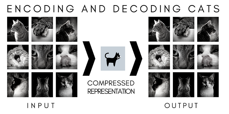
In this walk-through, we train an autoencoder model using a dataset of customers with good financial profiles that are seeking loans. The autoencoder will learn the common traits that make a customer a “good” credit risk. For example, it will remove outliers and rare events from the data. We then feed an out-of-sample dataset through this trained model — a set of customers with both good and bad credit. The trained autoencoder will reduce the data then rebuild it using the compressed representation back to its original size. Any customer that the model struggles to rebuild may potentially represent a red flag and require further investigation.

This is a great tool to better understand data. If you are unsure of what to focus on or you want to look at the big picture, an unsupervised or semi-supervised model might give you fresh insights and new areas to investigate.

Anomaly Detection and Autoencoders

Anomaly detection (or outlier detection) is the identification of items, events or observations which do not conform to an expected pattern or other items in a dataset — Wikipedia.com

Most deep learning models create additional features to better understand data, an autoencoder, on the other hand, reduces them. An autoencoder sheds information and ends with only a minimal set of weights or coefficients that still explains the data.

Autoencoding can also be seen as a non-linear alternative to PCA. It is similar to what we use in image, music, and file compression. It compresses the excess until the data is too distorted to be of value. This is all considered unsupervised learning, meaning the model isn’t looking for anything in particular, it simply tries to represent the data as accurately as possible in a reduced feature space.

This approach can be useful when you want to understand the common elements of your data. Not only will you better know who your “ideal” customer is, but it will also tell you who doesn’t conform. This may show you what bad credit risk looks like but may also highlight cases your business never knew about — like a segment of the population that requires a different intake process or set of measuring metrics to benefit from your services.

Actionable Insights and Autoencoders

At the end of the day, actionable insight is what data science is all about. If a company cannot apply the findings of a data science project, it is of no use to them.

An autoencoder is a fairly simple deep neural network. It will ingest the data set and, through a step of hidden layers, learn common and essential behavior and filter out the lesser ones. 

The Open Source Statlog — German Credit Data from the Data Set from the UC Irvine Machine Learning Repository

“This dataset classifies people described by a set of attributes as good or bad credit risks.”

UCI ML Repository

Let’s build an autoencoder with Python and Keras to learn what a “good” credit customer looks like by reducing the open-source Statlog-German Credit Data to its essential uniform elements. For the full source, see “Using Autoencoders and Keras to Better Understand your Customers”.

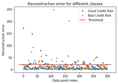
Once the model is trained, we take out-of-sample data and have the model predict (i.e. compress then reconstruct the data) and compare the error reconstruction value. The smaller the error, the closer the customer is to the “good” profile, the larger the error, the more anomalous it is.

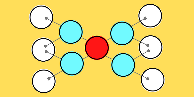
Let’s build our autoencoder. Building a model in Keras is very simple. You simply need to string each layer of your neural network one by one, then pass it to the “Model” function and it will set this all up for you automatically — long gone are the crazy Tensorflow 1.0 days where things were much, much more complicated. If you refer to the image above, we are going to follow a similar process, of taking the data in its original feature space, reduce a few times, then rebuild it again.

We’ll create an input layer to ingest the data then pass it through a dense layer with a Relu activation (rectified linear unit that will keep positive numbers and set any negative ones to zero) and the learning rate set earlier. We do that a few more times as we reduce the data then rebuild it. Finally, we pass it through the final dense layer with a linear activation that will output the data in its original dimension (prior to modeling).

# Autoencoder parameters
epochs = 500
batch_size = 128
input_dim = X_train_0.shape[1]
encoding_dim = 24
hidden_dim = int(encoding_dim / 2)
# select learning rate - if it doesn't converge try a bigger number
learning_rate = 1e-3

# Autoencoder layers
input_layer = Input(shape=(input_dim, ))
encoder = Dense(encoding_dim, activation="relu", activity_regularizer=regularizers.l1(learning_rate))(input_layer)
encoder = Dense(hidden_dim, activation="relu")(encoder)
decoder = Dense(hidden_dim, activation="relu")(encoder)
decoder = Dense(encoding_dim, activation="relu")(decoder)
decoder = Dense(input_dim, activation="linear")(decoder)
autoencoder = Model(inputs=input_layer, outputs=decoder)

Keras has a handy “summary()” function to quickly visualize what we build.

autoencoder.summary()
_________________________________________________________________
Layer (type)                 Output Shape              Param #   
=================================================================
input_3 (InputLayer)         [(None, 61)]              0         
_________________________________________________________________
dense_10 (Dense)             (None, 24)                1488      
_________________________________________________________________
dense_11 (Dense)             (None, 12)                300       
_________________________________________________________________
dense_12 (Dense)             (None, 12)                156       
_________________________________________________________________
dense_13 (Dense)             (None, 24)                312       
_________________________________________________________________
dense_14 (Dense)             (None, 61)                1525      
=================================================================
Total params: 3,781
Trainable params: 3,781
Non-trainable params: 0
_________________________________________________________________

Look at the “Output Shape” column and see the feature space going from 61, 24, 12, 12, 24, and finally back to 61 — that’s autoencoding.

We are ready to run the model using our credit data, this simply entails calling the Keras “fit()” function on our model.

autoencoder.fit(X_train_0, X_train_0,
                    epochs=epochs,
                    batch_size=batch_size,
                    shuffle=True,
                    validation_data=(X_test_0, X_test_0),
                    verbose=1,
                    callbacks=[cp, tb]).history

Mean Square Reconstruction Error

After running the trained model, we can run our out-of-sample set through it and get the mean square reconstruction error for each customer (each row). A large error may indicate credit risk. Compare the error rate of customer “818” versus “347”.

predictions = autoencoder.predict(X_test)
mse = np.mean(np.power(X_test - predictions, 2), axis=1)
print(mse)

507     20.325340
818    171.442944
452      3.171927
368      9.374798
242     13.166230
          ...    
459      3.613510
415      5.667701
61      21.307917
347      2.346015
349      7.616852
Length: 300, dtype: float64

We can find a reconstruction threshold that best represents the “good” versus “bad” credit risk. We can easily find that using Sklearn’s handy “roc_curve()” function.

fpr, tpr, thresholds = roc_curve(Y_test, mse)
print(‘thresholds’, np.mean(thresholds))

thresholds 21.05576286049008

Let’s Investigate!

We now have all we need to investigate some of the customers with large reconstruction errors. Remember, this is an unsupervised model that wasn’t trained to look at credit risk in particular (even if the data was made up of good risk only), instead, it may find anomalies anywhere — so this doesn’t mean that rows with high errors are automatically credit risks. 

Let’s create a subset of the data and look at the cases with high reconstruction error, what makes them different?

# What are some of those features that we see via poor reconstruction error?
X_test['Error'] = mse
X_test['CreditRisk'] = Y_test
X_test = X_test.sort_values('Error', ascending=False)
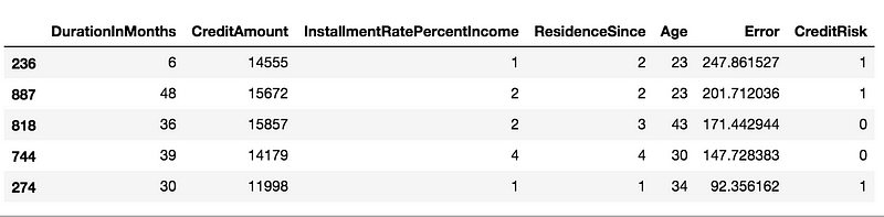
X_test[['DurationInMonths', 'CreditAmount', 'InstallmentRatePercentIncome', 
        'ResidenceSince', 'Age', 'Error', 'CreditRisk']].head()

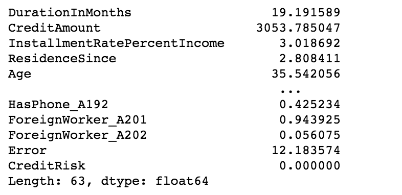
Let’s also take the mean of all the values for “good” credit so we can compare them against “normal” values.

normal_values = X_test[X_test['CreditRisk']==0].mean()
print(normal_values)

Customer “236”

The largest error of 247.9 belongs to the customer “236”. If we take the features that are the most positively anomalous compared to the mean of those same features for the entire cohort, we see:

Credit Amount: 14,555 DM
Duration In Months:  6

The mean credit amount requested is 3053 DM, this customer is asking for 10K over the mean — red flag? This customer also wants a loan for only 6 months while the cohort’s mean is 19 months.

Customer “887”

The second-largest reconstruction mean is customer “887”. The two most anomalous values are:

Credit Amount: 15,672 DM
Age  23

This customer is also requesting a large credit amount and is 12 years younger than the norm. 

Conclusion

I hope you understand how you can use an unsupervised model like the autoencoder to unearth interesting information and anomalies. This can be used to find credit risk just as it can be used to “unearth” new opportunities. The Keras code is loosely based on a great blog post from Chitta Ranjan “Extreme Rare Event Classification using Autoencoders in Keras”

You can find the full source code for this walk-through along with video companion at “Using Autoencoders and Keras to Better Understand your Customers”.

Thanks for reading!